KPConv (Kernel Point Convolution) is "a new design of point convolution, i.e. that operates on point clouds without any intermediate representation… KPConv is also efficient and robust to varying densities… and outperform state-of-the-art classification and segmentation approaches on several datasets" [6]

A point cloud is a set of data points in space usually produced by a Lidar sensor. Each data point in the set has several mandatory features - XYZ coordinate and some possible features; the color of the point (RGB), intensity, etc. Point clouds are useful for 3D modeling of objects, scanning large areas from aerial sensors, and autonomous vehicle scene understanding, among other things.

Figure 1: The first example is from the SemanticKitti dataset. The second example is from the Semantic3D dataset.

Most SOTA(state-of-the-art) models for classification and segmentation of images use CNNs (convolutional neural networks). However, point clouds' unique structure prevents us from using CNNs (we will discuss the differences in the following section). Therefore, an entire field of research arose trying to find deep learning solutions for processing point clouds.

The KPConv paper [6] introduces a novel NN layer that directly operates on point cloud data. It shows how to use this layer as part of a DNN for classification and segmentation tasks - achieving SOTA results.

This article will present how a KPConv layer works (both intuitively and mathematically) by diving into each module to fully understand this layer.

Challenges with point clouds

We can compare the structure of point clouds to images to understand the main challenges with point clouds. An image is a 2D grid of pixels where each pixel has a color (RGB). The distance between two adjacent pixels is always fixed. The order of the pixels determines the image's representation, i.e., a change in the pixels' order produces a new image. Moreover, there is extensive research on the classification and segmentation of images.

The complex structure of point cloud leads to four main challenges:

Sparse - The points are not evenly sampled in different regions.
Unstructured - Unlike images, point clouds are not placed on a grid. Each point is sampled independently, and its distance to its neighbors varies.
Unordered - As explained previously, a point cloud is represented by the XYZ coordinates. The order in which the points are stored does not alter the represented scene, so they are invariant to permutations.
Lack of research - there is no excessive research on it, compared to images, and the problem is far from being solved.

KPConv: flexible and deformable convolution for point clouds

The KPConv layer tries to overcome the explained challenges by creating a convolution[3] operation that works directly on the point cloud (without projecting the point cloud to a lower dimension).

Let's start with some intuition

The intuition behind KPConv is similar to the intuition behind CNNs. In CNN, each pixel is represented by a list of values known as 'channels' and is passed through k filters. The pixel's new representation is the dot product of neighboring pixel's channels (including the pixel itself) by the filters.

Similarly, in a KPConv layer, each point has fᵢ features (similar to channels) and is multiplied by k kernel points (similar to filters). The new representation of the point is the sum of all the kernel values multiplied by the neighbor's features.

General description

A KPConv layer is activated on every point in the point cloud. It gets a point (location and features) and its neighbors (location and features for each neighbor), and generates new features for the given point. The neighborhood of a point is defined by all the points located in a sphere with a fixed radius around a point. The neighbors' locations are centered (see ahead) on the given point (XYZ values of each neighbor are centered relative to the given point location), similar to a convolution layer filter.

A KPConv layer is defined by several kernel points (similar to filters in CNN). The kernel points are positioned regularly (See Figure 3) in a sphere around the given point (i.e., each point tries to be as far as possible from any other point and still stays in the sphere around the center). Each kernel point has a set of weights (similar to filters), which are applied to the neighboring points. Each kernel point's weights are applied to the neighboring points relative to the distance between the kernel point and the neighbor. Thus, each kernel point has an area of influence defined by a correlation function (see ahead). The correlation function defines whether a kernel point influences a point and how the neighbor point contributes to calculating the kernel value.

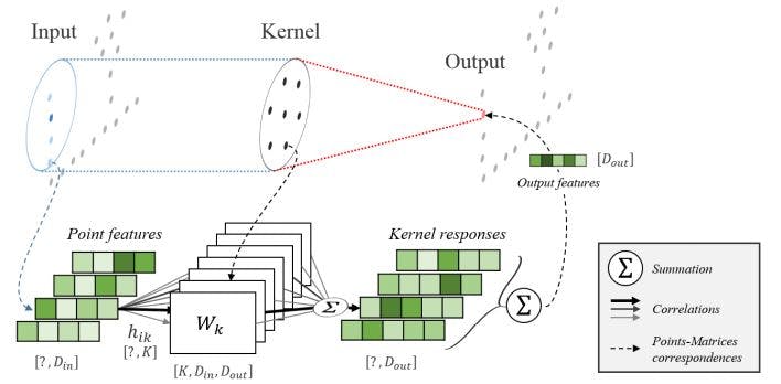kernel points correlations.JPG Figure 2: An illustration of a neighboring point to each kernel point correlations.

The given point's new features are calculated as the sum of all the neighbors' features multiplied by their correlation and learned weights. At the input layer, each point's features are set to the point's attributes, such as RGB, intensity, etc. In a way analogous to input RGB channels to a CNN. After the first operation of the KPConv layer on the point cloud, each point has new features (similar to channels in CNN), which are used to calculate the next layer of KPConv.

In the following sections, I will present a full description of each sub-part of the KPConv layer.

Rigid kernel

"The convolution weights of KPConv are located in Euclidean space by kernel points, and applied to the input points close to them." [6]

The kernel points are points that are regularly positioned around each point in the point cloud. Each kernel point has a weight matrix and is applied to each point's close neighbors in the point cloud.

The kernel points' locations are determined by solving an optimization problem. The kernel points need to be as far as possible from one another but as close as possible to the center (which is the location of the given point). One of the points is constrained to be at the center. The rigid kernel is related to kernel points, which are arranged regularly in a sphere. These are examples of kernel point locations with different K values: 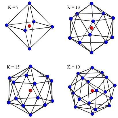Kernel points.png Figure 3: The blue points are the kernel points, and the red point is the center of the sphere, which is the given point to the KPConv layer (one of the kernel points is placed in the center).

The use of multiple kernel points allows distinguishing information from different directions of the processed point's neighboring. The regular arrangement of the kernel point produces uniform resolution in each direction.

Similar to CNN, where each kernel has a set of weights with the shape of the input channels and the output channels, each kernel point has a unique set of weights with the shape of [fᵢₙ,fₒᵤₜ], where fᵢₙ is the number of features of the point in the current layer and fₒᵤₜ is the number of features in the next layer.

Kernel function

"kernel function g, which is where KPConv singularity lies."

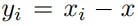
The kernel function takes a neighbor position xᵢ and centers it on the given point x. The centered position of neighbor xᵢ is calculated by:

According to the neighbor location, the kernel function g(yᵢ) applies a different ratio (correlation) to the kernel weights. The kernel value for a given neighbor is calculated as a weighted sum of all the kernel weights with the kernel correlations:

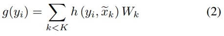
where h(yᵢ, xₖ) is a correlation function that will be explained later, xₖ is the kernel point location and Wₖ is the weight matrix of kernel k.

The kernel value that is calculated for each neighbor yᵢ is then multiplied by the neighbor features fᵢ :

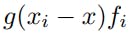
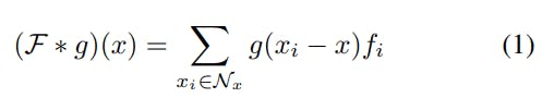
The new representation of the given point x is calculated as the sum of all the kernel values of x's neighbors:

Correlations

The correlation function calculates the correlation between each neighbor xᵢ and a kernel point xₖ. The correlations are used to weigh each kernel's contribution to the total kernel value of each neighbor. The correlation is calculated according to the locations of each point (XYZ).

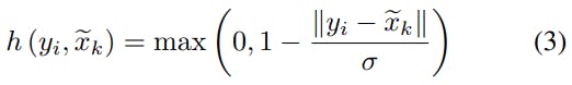
Where σ is a hyper-parameter that is defined as the influence distance of the kernel points. The density of the point cloud determines this hyper-parameter.

This correlation function provides higher values when the points are close to each other, and its value is between [0,1]. These are two fundamental requirements they declared for the correlation function.

Assemble All - with mathematics

For a batch size of n points. Every point has a maximum of nₙₑᵢ neighbors. k is the number of kernel points. The features of each point are represented by fᵢ. neighb_x are the features of each neighborhood (dim(neighb_x)=[n,nₙₑᵢ,fᵢ]). kernel_weights are the weights of each kernel point. dim(kernel_weights)=[k,fᵢₙ,fₒᵤₜ].

Center each neighborhood dim(neighbors) = [n,nₙₑᵢ,3].
Calculate the differences between each neighborhood and kernel points: diffs = neighbors-kernels. dim(kernels)=[k,3], dim(diffs)=[n,nₙₑᵢ,k,3].
Calculate the correlation by applying L1 norm to the differences and sum the differences along the 4ᵗʰ axis (XYZ axis). correlations=min(1-Σ||diffs||/σ, 0). dim(correlations)=[n,k,nₙₑᵢ].
The new representation of each point is calculated the following way: new_representation=Σ(correlationsneighb_x)ᵀkernel_weights. dim(new_representation)=[n,fₒᵤₜ]

Deformable kernel

"…deformable version of our convolution, which consists of learning local shifts applied to the kernel points."

Similar to deformable CNN[4], KPConv implements a deformable version. The deformable version of KPConv generates shifts for each kernel point, which are added to each location of the kernel point to determine their new locations. The function △(x) generates k shifts based on the given point. Each shift contains three values (one value for each axis), i.e. △(x) generates 3k values and are reshaped to (3,k). The shifts are calculated according to the area of the given point x.

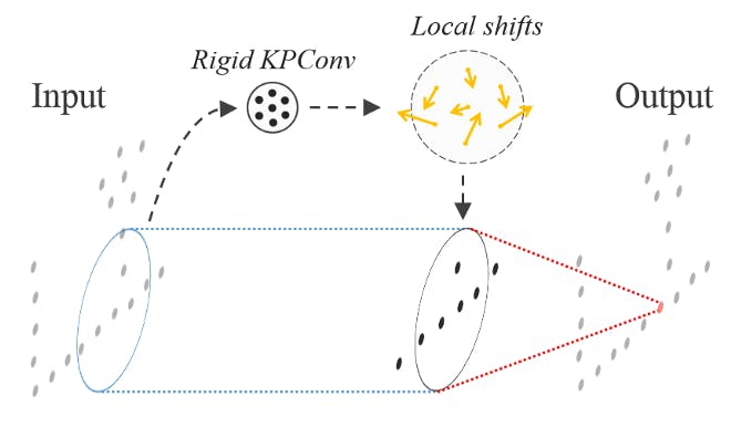Figure 4: Deformable Convolution with shifts calculation

The changes that are needed to be made to use the deformable version are in the main KPConv function and the kernel function:

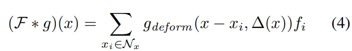
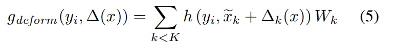
The offset function △(x) is calculated by a rigid KPConv layer with the same input parameters as the deformable parameters, and the output dimension is 3K. The output of △(x) is reshaped to (K,3) and is used to calculate the new location of each kernel point. Each kernel point's new location is calculated as the sum of the original location (similar to the rigid version) and the calculated shifts.

How KPConv handles point cloud's challenges?

Sparse - As shown in[5], radius neighborhoods provide robustness to varying densities compared to KNN neighborhoods. KPConv layer samples neighborhoods using a per-dataset radius.
Unstructured - KPConv creates a sphere around each point in the point cloud, which reduces the importance of the neighborhood's inner structure and increases the importance of the relations between the neighbors and the kernel points.
Unordered - KPConv layer doesn't give importance to the order of the points. It looks at each point's features and its neighborhood features to generate new embedding.

Conclusion

In this post, I explained the challenges we face when working with point clouds and how a KPConv layer overcome those challenges. Most of the existing methods project the point cloud to an intermediate representation, which can cause loss of information when processing the input. KPConv presents an elegant approach for processing point clouds that has similar logic to CNN.

References

[1] arxiv.org/pdf/2001.06280.pdf
[2] mdpi.com/2072-4292/12/11/1729/htm
[3] en.wikipedia.org/wiki/Convolutional_neural_..
[4] towardsdatascience.com/deformable-convoluti..